JEE Physics Formula Booklet

1. UNIT AND DIMENSIONS

Unit: Measurement of any physical quantity is expressed in terms of an internationally accepted certain basic standard called unit.

Fundamental Units

S.No.	Physical Quantity	SI Unit	Symbol
1	Length	Metre	m
2	Mass	Kilogram	Kg
3	Time	Second	S
4	Electric Current	Ampere	A
5	Temperature	Kelvin	K
6	Luminous Intensity	Candela	Cd
7	Amount of Substance	Mole	mol

Supplementary Units

S.No.	Physical Quantity	SI Unit	Symbol
1	Plane Angle	radian	r
2	Solid Angle	Steradian	Sr

Metric Prefixes

S.No.	Prefix	Symbol	Value
1	Centi	c	10^-2
2	Milli	m	10^-3
3	Micro	µ	10^-6
4	Nano	n	10^-9
5	Pico	p	10^-12
6	Kilo	K	10³
7	Mega	M	10⁶

2. RECTILINEAR MOTION

Average Velocity (in an interval):

\[v_{av} = \bar{v} = \langle v \rangle = \frac{\text{Total displacement}}{\text{Total time taken}} = \frac{\vec{r}_f - \vec{r}_i}{\Delta t}\]

Average Speed (in an interval)

\[\text{Average Speed} = \frac{\text{Total distance travelled}}{\text{Total time taken}}\]

Instantaneous Velocity (at an instant):

\[\bar{v}_{\text{inst}} = \lim_{\Delta t \to 0} \left( \frac{\Delta \vec{r}}{\Delta t} \right)\]

Average acceleration (in an interval):

\[\vec{a}_{av} = \frac{\Delta \bar{v}}{\Delta t} = \frac{\bar{v}_f - \bar{v}_i}{\Delta t}\]

Instantaneous Acceleration (at an instant):

\[\vec{a} = \frac{d\bar{v}}{dt} = \lim_{\Delta t \to 0} \left( \frac{\Delta v}{\Delta t} \right)\]

Graphs in Uniformly Accelerated Motion along a straight line (a ≠ 0)

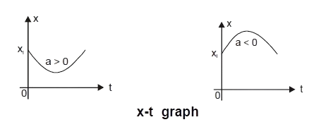
\( x \) is a quadratic polynomial in terms of \( t \). Hence \( x - t \) graph is a parabola.
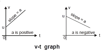
\( v \) is a linear polynomial in terms of \( t \). Hence \( v - t \) graph is a straight line of slope \( a \).
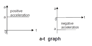
a-t graph is a horizontal line because a is constant.

Maxima & Minima

\[\frac{dy}{dx} = 0 \quad \& \quad \frac{d}{dx} \left( \frac{dy}{dx} \right) < 0 \quad \text{at maximum}\] \[\text{and} \quad \frac{dy}{dx} = 0 \quad \& \quad \frac{d}{dx} \left( \frac{dy}{dx} \right) > 0 \quad \text{at minima.}\]

Equations of Motion (for constant acceleration)

(a) \( v = u + at \)

(b) \( s = ut + \frac{1}{2} at^2 \quad s = vt - \frac{1}{2} at^2 \quad \)

\( x_t = x_i + ut + \frac{1}{2} at^2 \)

(d) \( s = \frac{(u + v)}{2} t \)

(e) \( s_n = u + \frac{a}{2} (2n - 1) \)

For freely falling bodies : (\( u = 0 \)) (taking upward direction as positive)

(a) \( v = -gt \)

(b) \( s = -\frac{1}{2} gt^2 \quad s = vt + \frac{1}{2} gt^2 \quad h_t = h_1 - \frac{1}{2} gt^2 \)

(d) \( s_n = -\frac{g}{2} (2n - 1) \)

3. PROJECTILE MOTION & VECTORS

Time of flight:

\[ T = \frac{2u\sin\theta}{g} \]

Horizontal range:

\[ R = \frac{u^2 \sin 2\theta}{g} \]

Maximum height:

\[ H = \frac{u^2 \sin^2\theta}{2g} \]

Trajectory equation (equation of path):

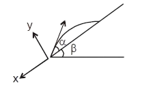
\[ y = x \tan \theta - \frac{gx^2}{2u^2 \cos^2 \theta} = x \tan \theta \left( 1 - \frac{x}{R} \right) \]

Projection on an inclined plane

	Up the Incline	Down the Incline
Range	\(\frac{2u^2 \sin \alpha \cos(\alpha + \beta)}{g \cos^2 \beta}\)	\(\frac{2u^2 \sin \alpha \cos(\alpha - \beta)}{g \cos^2 \beta}\)
Time of flight	\(\frac{2u \sin \alpha}{g \cos \beta}\)	\(\frac{2u \sin \alpha}{g \cos \beta}\)
Angle of projection with incline plane for maximum range	\(\frac{\pi}{4} - \frac{\beta}{2}\)	\(\frac{\pi}{4} + \frac{\beta}{2}\)
Maximum Range	\(\frac{u^2}{g(1 + \sin \beta)}\)	\(\frac{u^2}{g(1 - \sin \beta)}\)

4. RELATIVE MOTION

\[ \vec{V}_{AB} \text{ (velocity of A with respect to B)} \]

\[ = \vec{V}_A - \vec{V}_B \]

\[ \vec{a}_{AB} \text{ (acceleration of A with respect to B)} \]

\[ = \vec{a}_A - \vec{a}_B \]

Relative motion along straight line:

\[ \vec{x}_{BA} = \vec{x}_B - \vec{x}_A \]

CROSSING RIVER

A boat or man in a river always moves in the direction of resultant velocity of velocity of boat (or man) and velocity of river flow.

1. Shortest Time:

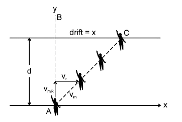
Velocity along the river, \( v_x = v_R \)

Velocity perpendicular to the river, \( v_t = v_{mR} \)

The net speed is given by

\[ v_m = \sqrt{v_{mR}^2 + v_R^2} \]

2. Shortest Path:

velocity along the river, \( v_x = 0 \)

and velocity perpendicular to river

\[ v_y = \sqrt{v_{mR}^2 - v_R^2} \]

The net speed is given by

\[ v_m = \sqrt{v_{mR}^2 - v_R^2} \]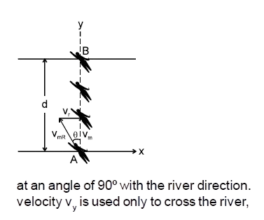

Therefore time to cross the river, \( t = \frac{d}{v_y} = \frac{d}{\sqrt{v^2_{mR} - v^2_R}} \)

and velocity \( v_x \) is zero, therefore, in this case the drift should be zero.

\[ \Rightarrow v_R - v_{mR} \sin \theta = 0 \quad \text{or} \quad v_R = v_{mR} \sin \theta \] \[ \text{or} \quad \theta = \sin^{-1} \left( \frac{v_R}{v_{mR}} \right) \]

RAIN PROBLEMS

\[ \bar{v}_{Rm} = \bar{v}_R - \bar{v}_m \quad \text{or} \quad v_{Rm} = \sqrt{v^2_R + v^2_m} \]

5. NEWTON'S LAWS OF MOTION

1. From third law of motion

\[ \vec{F}_{AB} = -\vec{F}_{BA} \] \[ \vec{F}_{AB} = \text{Force on A due to B} \] \[ \vec{F}_{BA} = \text{Force on B due to A} \]

2. From second law of motion

\[ F_x = \frac{dP_x}{dt} = ma_x \quad F_y = \frac{dP_y}{dt} = ma_y \quad \]

\[ F_z = \frac{dP_z}{dt} = ma_z \]

5. WEIGHING MACHINE:

A weighing machine does not measure the weight but measures the force exerted by object on its upper surface.

6. SPRING FORCE

\[ \vec{F} = -\vec{kx} \]

\( x \) is displacement of the free end from its natural length or deformation of the spring where \( K = \) spring constant.

7. SPRING PROPERTY

\[ K \times \ell = \text{constant} = \text{Natural length of spring} \]

8. If spring is cut into two in the ratio \( m : n \) then spring constant is given by

\[ \ell_1 = \frac{m\ell}{m+n}; \quad \ell_2 = \frac{n\ell}{m+n} \quad k\ell = k_1\ell_1 = k_2\ell_2 \]

For series combination of springs

\[ \frac{1}{k_{eq}} = \frac{1}{k_1} + \frac{1}{k_2} + \ldots \]

For parallel combination of spring

\[ k_{eq} = k_1 + k_2 + k_3 \ldots \]

9. SPRING BALANCE:

It does not measure the weight. It measures the force exerted by the object at the hook.

Remember: physics formulas

11.

12. WEDGE CONSTRAINT:

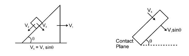
Components of velocity along perpendicular direction to the contact plane of the two objects is always equal if there is no deformations and they remain in contact.

13. NEWTON'S LAW FOR A SYSTEM

\[ \vec{F}_{\text{ext}} = \]

\[ m_1 \vec{a}_1 + m_2 \vec{a}_2 + m_3 \vec{a}_3 + \ldots \]

\[ \vec{F}_{\text{ext}}= \]

\[ \text{Net external force on the system} \]

\[ m_1, \, m_2, \, m_3 \, \]

\[ \text{are the masses of the objects of the system and} \]

\[ \vec{a}_1, \, \vec{a}_2, \, \vec{a}_3 \, \]

\[ \text{are the acceleration of the objects respectively} \]

14. NEWTON'S LAW FOR NON INERTIAL FRAME:

\[ \vec{F}_{\text{Real}} + \vec{F}_{\text{Pseudo}} = m\vec{a} \]

Net sum of real and pseudo force is taken in the resultant force.

\[ \vec{a} = \]

Acceleration of the particle in the non inertial frame

\[ \vec{F}_{\text{Pseudo}} = -m \, \vec{a}_{\text{Frame}} \]

(a) Inertial reference frame: Frame of reference moving with constant velocity.

(b) Non-inertial reference frame: A frame of reference moving with non-zero acceleration.

6. FRICTION

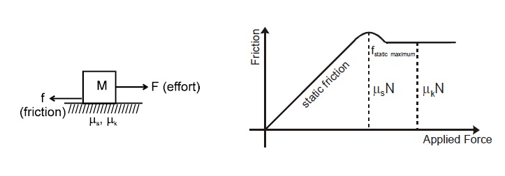
Friction force is of two types:

Kinetic
Static

Kinetic Friction:

\[ f_k = \mu_k N \]

The proportionality constant \( \mu_k \) is called the coefficient of kinetic friction.

Static Friction:

It exists between two surfaces when there is tendency of relative motion but no actual motion.

This means static friction is a variable and self adjusting force.However it has a maximum value called limiting friction.

\[ f_{\text{max}} = \mu_s N \] \[ 0 \leq f_s \leq f_{\text{smax}} \]

7. WORK, POWER & ENERGY

WORK DONE BY CONSTANT FORCE:

\[ W = \vec{F} \cdot \vec{S} \]

WORK DONE BY MULTIPLE FORCES

\[ \Sigma \vec{F} = \vec{F}_1 + \vec{F}_2 + \vec{F}_3 + \ldots \] \[ W = [\Sigma \vec{F}] \cdot \vec{S} \] or \[ W = \vec{F}_1 \cdot \vec{S} + \vec{F}_2 \cdot \vec{S} + \vec{F}_3 \cdot \vec{S} + \ldots \] \[ W = W_1 + W_2 + W_3 + \ldots \]

WORK DONE BY A VARIABLE FORCE

\[ dW = \vec{F} \cdot d\vec{S} \]

RELATION BETWEEN MOMENTUM AND KINETIC ENERGY

\[ K = \frac{p^2}{2m} \quad \text{and} \quad P = \sqrt{2mK} \]

where \( P \) = linear momentum

POTENTIAL ENERGY

\[ \int_{U_1}^{U_2} dU = -\int_{r_1}^{r_2} \vec{F} \cdot d\vec{r} \] \[ U_2 - U_1 = -\int_{r_1}^{r_2} \vec{F} \cdot d\vec{r} = -W \] \[ U = -\int_{\infty}^{r} \vec{F} \cdot d\vec{r} = -W \]

CONSERVATIVE FORCES

\[ F = -\frac{\partial U}{\partial r} \]

WORK-ENERGY THEOREM

\[ W_C + W_{NC} + W_{PS} = \Delta K \]

Modified Form of Work-Energy Theorem:

\[ W_C = -\Delta U \] \[ W_{NC} + W_{PS} = \Delta K + \Delta U \] \[ W_{NC} + W_{PS} = \Delta E \]

POWER

The average power (\( \overline{P} \) or \( p_{av} \)) delivered by an agent is given by:

\[ \overline{P} = \frac{W}{t} \] \[ P = \frac{\vec{F} \cdot d\vec{S}}{dt} = \vec{F} \cdot \frac{d\vec{S}}{dt} = \vec{F} \cdot \vec{v} \]

8. CIRCULAR MOTION

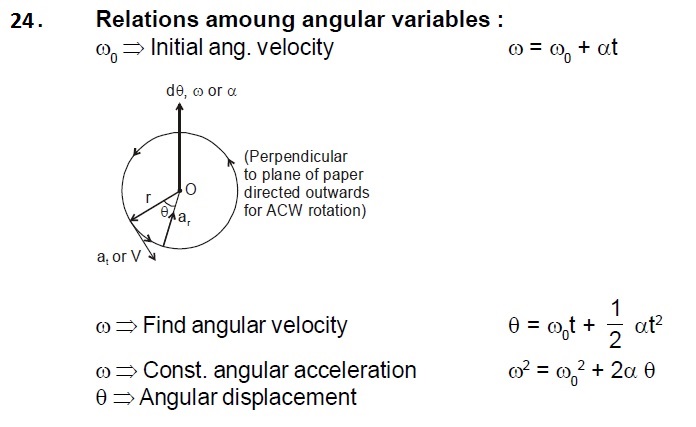
1. Average angular velocity

\[ \omega_{av} = \frac{\theta_2 - \theta_1}{t_2 - t_1} = \frac{\Delta \theta}{\Delta t} \]

2. Instantaneous angular velocity

\[ \omega = \frac{d\theta}{dt} \]

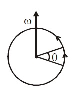
3. Average angular acceleration

\[ \alpha_{av} = \frac{\omega_2 - \omega_1}{t_2 - t_1} = \frac{\Delta \omega}{\Delta t} \]

4. Instantaneous angular acceleration

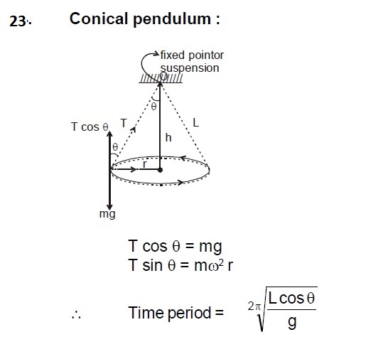
\[ \alpha = \frac{d\omega}{dt} = \omega \frac{d\omega}{d\theta} \]

5. Relation between speed and angular velocity

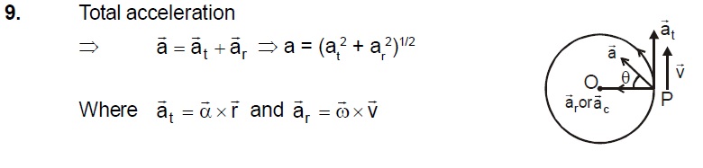
\[ v = r\omega \quad \text{and} \quad \vec{v} = \vec{\omega} \times \vec{r} \]

7. Tangential acceleration (rate of change of speed)

\[ a_t = \frac{dV}{dt} = r \frac{d\omega}{dt} = \omega \frac{dr}{dt} \]

8. Radial or normal or centripetal acceleration

\[ a_r = \frac{V^2}{r} = \omega^2 r \]

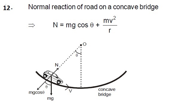
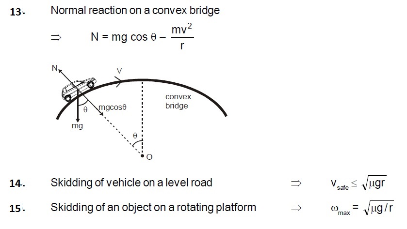
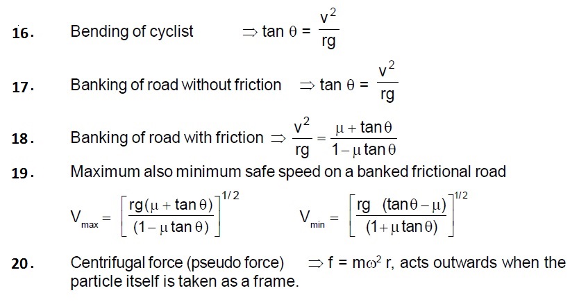
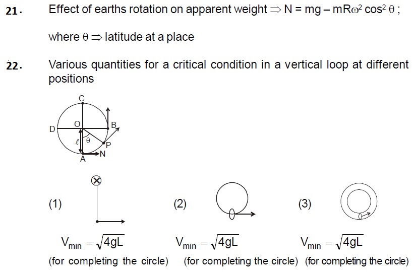
9. CENTRE OF MASS

Mass Moment:

\[ \tilde{M} = m \tilde{r} \]

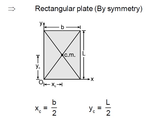
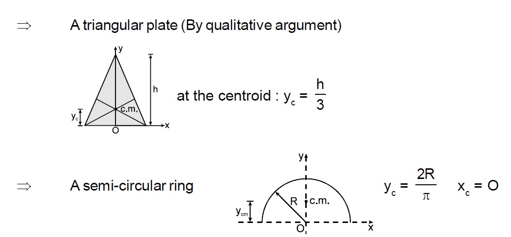
CENTRE OF MASS OF A SYSTEM OF 'N' DISCRETE PARTICLES

\[ \vec{r}_{\text{cm}} = \frac{m_1 \vec{r}_1 + m_2 \vec{r}_2 + \ldots + m_n \vec{r}_n}{m_1 + m_2 + \ldots + m_n} \] \[ \sum_{i=1}^{n} m_i \vec{r}_i = \frac{1}{M} \sum_{i=1}^{n} m_i \vec{r}_i \]

CENTRE OF MASS OF A CONTINUOUS MASS DISTRIBUTION

\[ x_{cm} = \frac{\int x dm}{\int dm}, \quad y_{cm} = \frac{\int y dm}{\int dm}, \quad z_{cm} = \frac{\int z dm}{\int dm} \]

where \( \int dm = M \) (mass of the body)

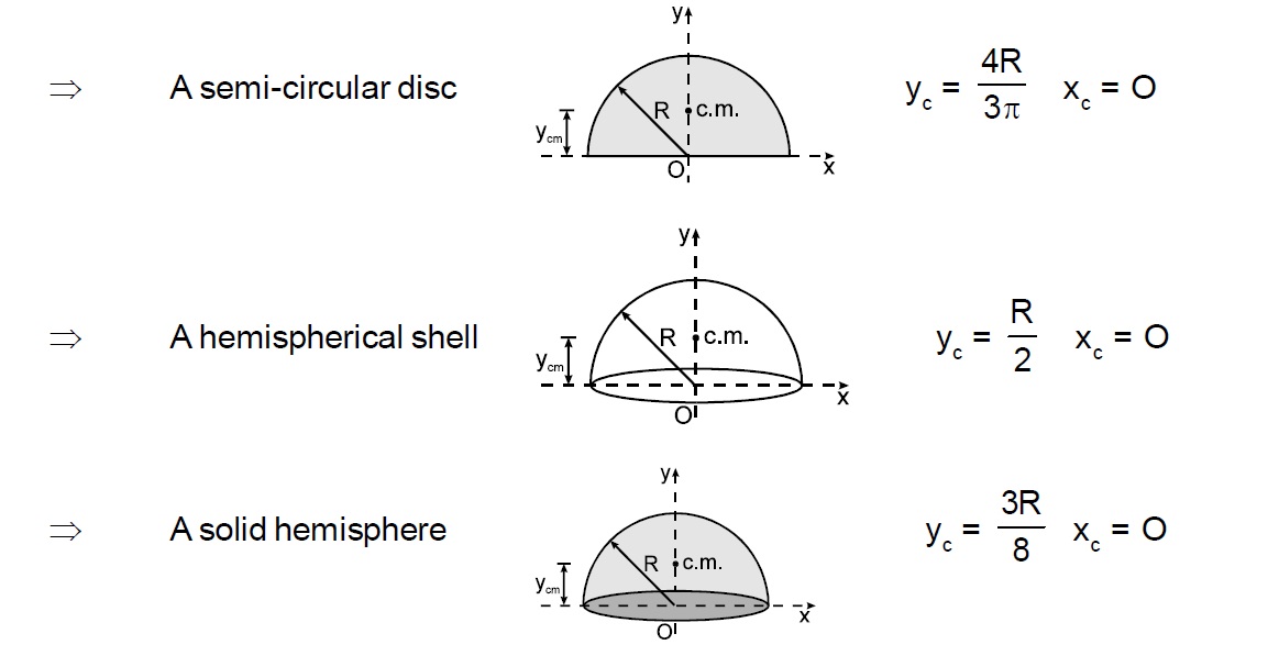
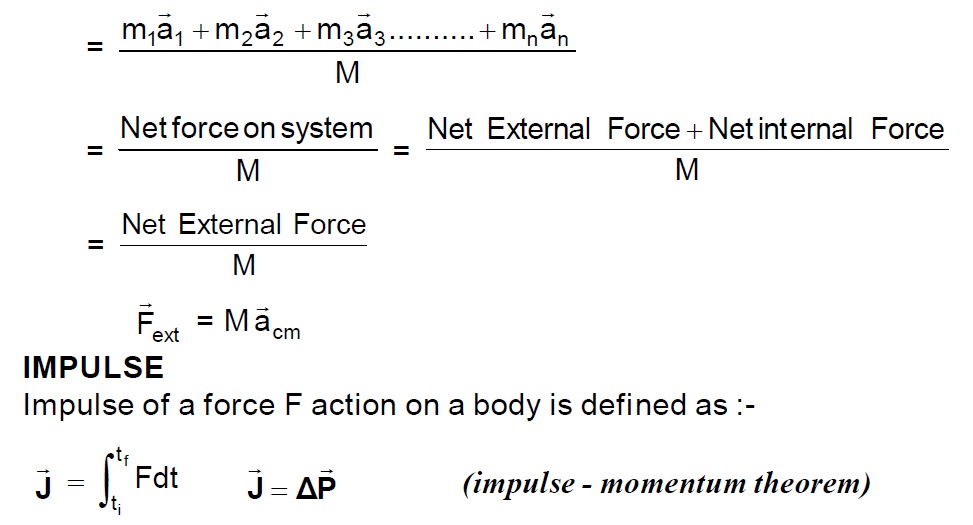
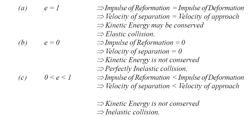
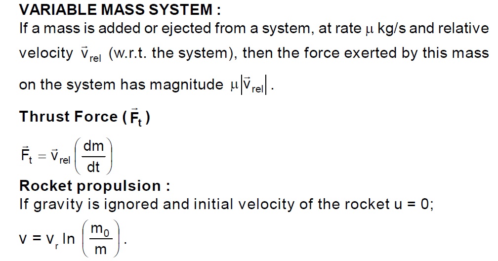
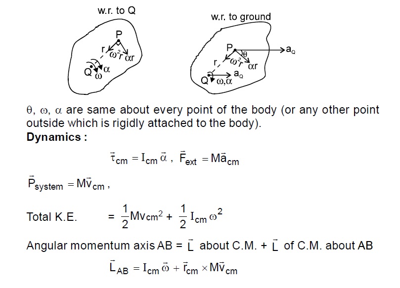
10. RIGID BODY DYNAMICS

1. RIGID BODY:

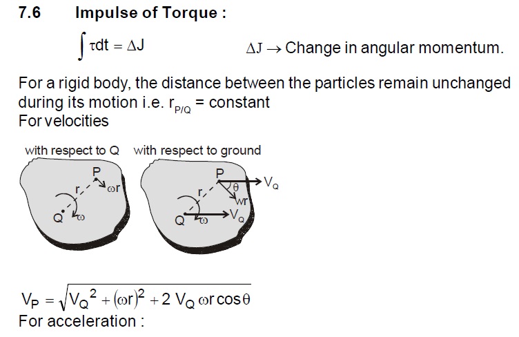
A rigid body is one for which the distance between any two particles of the body remains constant.

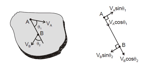
For a rigid body, if points A and B are part of the same rigid body:

\[ V_A \cos \theta_1 = V_B \cos \theta_2 \] \[ V_{AB} = \text{relative velocity of point B with respect to point A} \]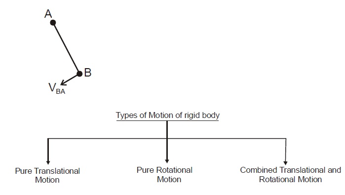

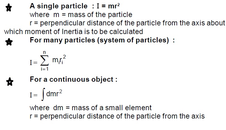
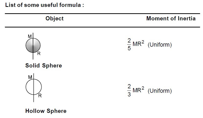
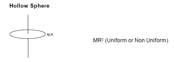
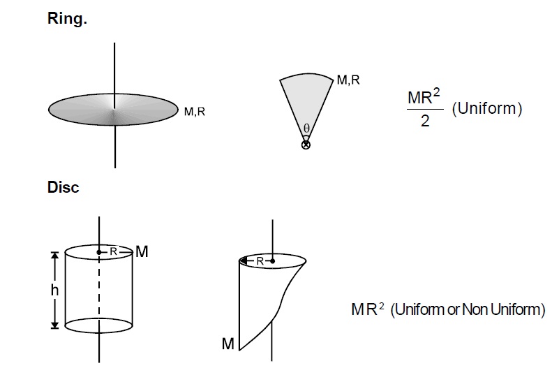
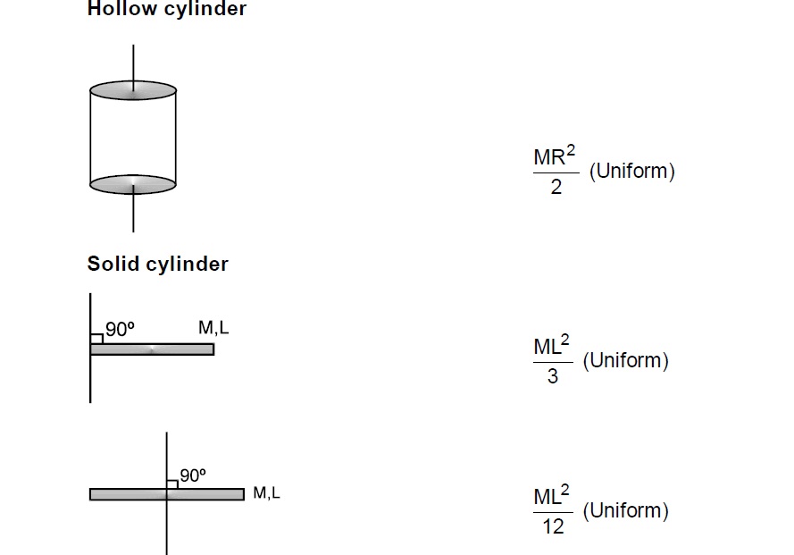
2. MOMENT OF INERTIA (I):

Definition: Moment of Inertia is defined as the capability of system to oppose the change produced in the rotational motion of a body.

Moment of Inertia is a scalar positive quantity.

I = m₁r₁^{2 + m₂r₂² + ..............}

= I₁ + I₂ + I₃ + ..................

SI units of Moment of Inertia is Kgm2.

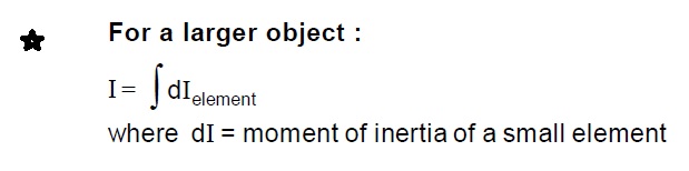
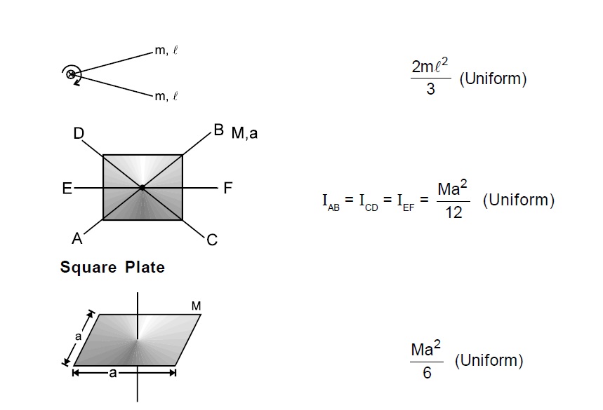
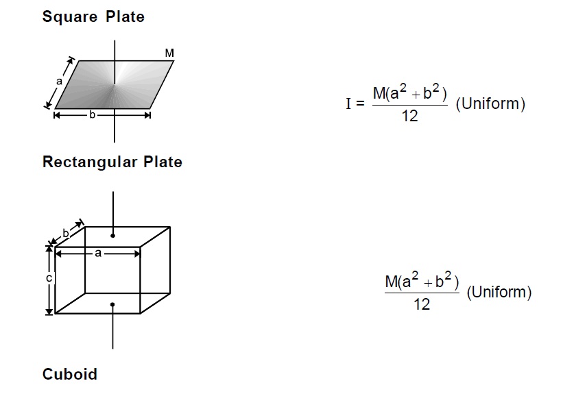
Moment of Inertia of :

3. TWO IMPORTANT THEOREMS ON MOMENT OF INERTIA:

3.1 Perpendicular Axis Theorem

[Only applicable to plane lamina (2-D objects)]

\[ I_z = I_x + I_y \quad \text{(when object is in x-y plane)} \]

3.2 Parallel Axis Theorem

(Applicable to any type of object):

\[ I_{AB} = I_{cm} + Md^2 \]

4. RADIUS OF GYRATION:

\[ I = MK^2 \]

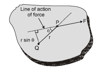
5. TORQUE:

\[ \tau = r \times \vec{F} \]

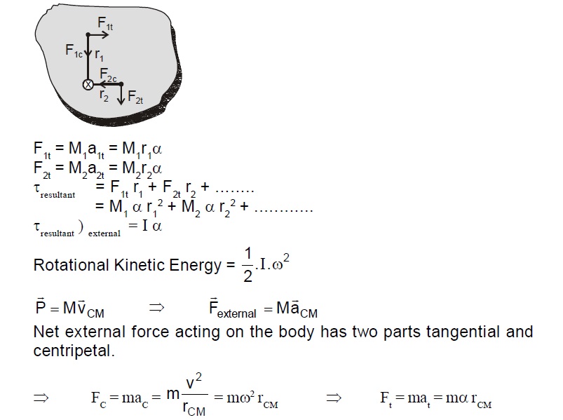
Relation between torque and angular acceleration:

\[ \vec{\tau}_{\text{ext}} / \text{hinge} = I_{\text{hinge}} \vec{\alpha} \]

Where \( \vec{\tau}_{\text{ext}} / \text{hinge} \) = net external torque acting on the body about hinge point

\( I_{\text{Hinge}} \) = moment of inertia of body about hinge point

6. ROTATIONAL EQUILIBRIUM:

For translational equilibrium:

\[ \sum F_x = 0 \] \[ \sum F_y = 0 \]

The condition of rotational equilibrium is:

\[ \sum \tau_z = 0 \]

7. ANGULAR MOMENTUM (L)

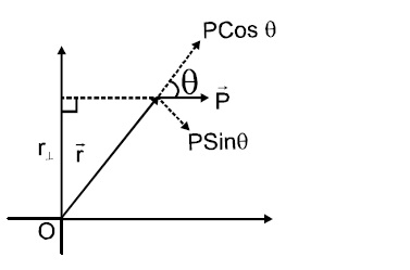
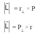
7.1 Angular momentum of a particle about a point:

\[ \vec{L} = \vec{r} \times \vec{p} \] \[ L = rp \sin \theta \] physics formulas

7.3 Angular momentum of a rigid body rotating about fixed axis:

\[ \vec{L} = I \vec{\omega} \] \[ L_H = \text{angular momentum of object about axis H.} \] \[ I_H = \text{Moment of Inertia of rigid object about axis H.} \] \[ \omega = \text{angular velocity of the object.} \]

7.4 Conservation of Angular Momentum:

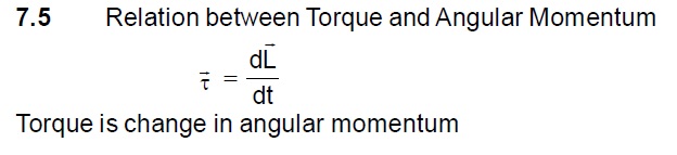
Angular momentum of a particle or a system remains constant if \( \tau_{ext} = 0 \) about that point or axis of rotation.

11. SIMPLE HARMONIC MOTION

\[ F = -kx \]

General equation of S.H.M. is:

\[ x = A \sin (\omega t + \phi) \]

where \((\omega t + \phi)\) is phase of the motion and \(\phi\) is initial phase.

Angular Frequency (\(\omega\)):

\[ \omega = \frac{2\pi}{T} = 2\pi f \]

Time period (T):

\[ T = \frac{2\pi}{\omega} = 2\pi \sqrt{\frac{m}{k}} \]

Speed:

\[ v = \omega \sqrt{A^2 - x^2} \]

Acceleration:

\[ a = -\omega^2 x \]

Energy Relations:

Kinetic Energy (KE):

\[ \frac{1}{2} mv^2 = \frac{1}{2} m\omega^2 (A^2 - x^2) = \] \[ \frac{1}{2} k (A^2 - x^2) \]

Potential Energy (PE):

\[ \frac{1}{2} kx^2 \]

Total Mechanical Energy (TME):

\[ = K.E. + P.E. = \frac{1}{2} k (A^2 - x^2) + \frac{1}{2} kx^2 = \] \[ \frac{1}{2} kA^2 \text{ (constant)} \]

SPRING-MASS SYSTEM

(1) Basic system:

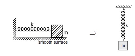\[ T = 2\pi \sqrt{\frac{m}{k}} \]

(2) Two masses:

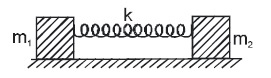\[ \tau = 2\pi \sqrt{\frac{\mu}{k}}, \text{ where } \mu = \] \[ \frac{m_1 m_2}{(m_1 + m_2)} \text{ (reduced mass)} \]

COMBINATION OF SPRINGS

Series Combination:

\[ \frac{1}{k_{eq}} = \frac{1}{k_1} + \frac{1}{k_2} \]

Parallel Combination:

\[ k_{eq} = k_1 + k_2 \]

SIMPLE PENDULUM

\[ T = 2\pi \sqrt{\frac{\ell}{g}} \]

In accelerating reference frame; \( g_{\text{eff}} \) is net acceleration due to pseudo force and gravitational force.

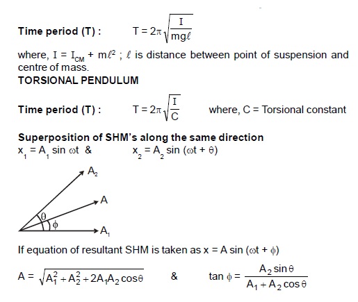
COMPOUND PENDULUM / PHYSICAL PENDULUM

Damped Oscillations

Damping force:

\[ F = -bv \]

Equation of motion:

\[ m \frac{dv}{dt} = -kx - bv \] \[ b^2-4mk>0 \text{ over damping} \] \[ b^2-4mk=0 \text{ critical damping} \] \[ b^2-4mk<0 \text{ under damping} \]

Solution for underdamped case:

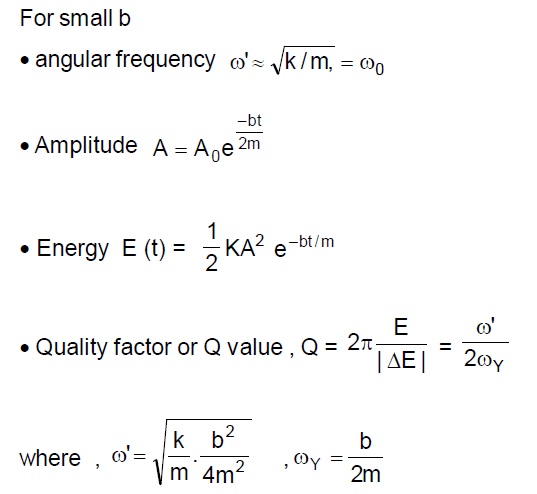
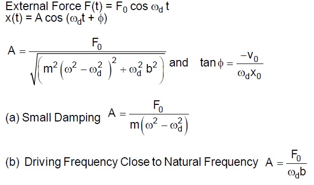
\[ x = \left( A_0 e^{-bt/2m} \right) \sin [\omega' t + \delta] \] \[ \omega' = \sqrt{\left( \frac{k}{m} \right) - \left( \frac{b}{2m} \right)^2} \] physics formulas

Forced Oscillations And Resonance

12. STRING WAVE

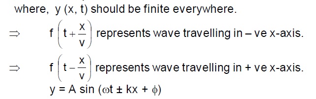
GENERAL EQUATION OF WAVE MOTION:

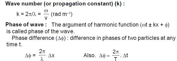
\[ \frac{\partial^2 y}{\partial t^2} = v^2 \frac{\partial^2 y}{\partial x^2} \] \[ y(x,t) = f \left( t \pm \frac{x}{v} \right) \] physics formulas

TERMS RELATED TO WAVE MOTION ( FOR 1-D PROGRESSIVE SINE WAVE )

SPEED OF TRANSVERSE WAVE ALONG A STRING/WIRE:

\[ v = \sqrt{\frac{T}{\mu}} \]

where \( T \) = Tension, \( \mu \) = mass per unit length

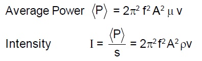
POWER TRANSMITTED ALONG THE STRING BY A SINE WAVE

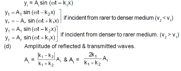
REFLECTION AND REFRACTION OF WAVES

STANDING WAVES:

For two waves:

\[ y_1 = A \sin (\omega t - kx + \theta_1) \] \[ y_2 = A \sin (\omega t + kx + \theta_2) \] \[ y_1 + y_2 = \] \[ \left[ 2 A \cos \left( kx + \frac{\theta_2 - \theta_1}{2} \right) \right] \sin \left( \omega t + \frac{\theta_1 + \theta_2}{2} \right) \]

The quantity \[ 2 A \cos \left( kx + \frac{\theta_2 - \theta_1}{2} \right) \] represents resultant amplitude at x. At some position resultant amplitude is zero these are called nodes.At some positions resultant amplitude is 2A, these are called antinodes.

Properties:

Distance between successive nodes or antinodes = \(\frac{\lambda}{2}\)
Distance between successive nodes and antinodes = \(\frac{\lambda}{4}\)
All particles in same segment (portion between two successive nodes) vibrate in same phase
Particles in consecutive segments vibrate in opposite phase
Since nodes are permanently at rest so energy can not be transmitted across these.

VIBRATIONS OF STRINGS (STANDING WAVE)

Fixed at both ends:

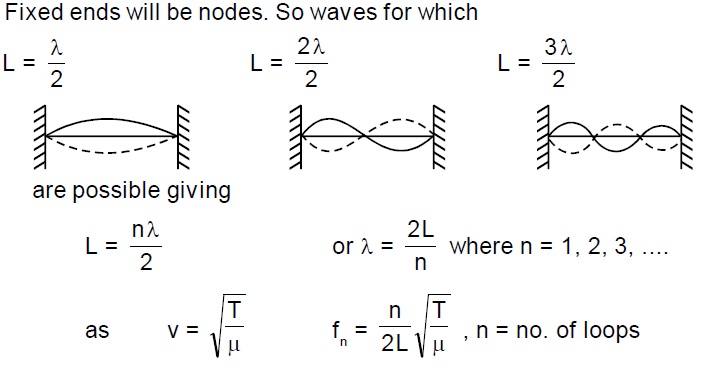
String free at one end:

13. HEAT & THERMODYNAMICS

Kinetic Theory of Gases:

Total translational K.E. of gas:

\[ \frac{1}{2} M \langle V^2 \rangle = \frac{3}{2} PV = \frac{3}{2} nRT \]

Root mean square speed:

\[ V_{\text{rms}} = \sqrt{\frac{3P}{\rho}} = \sqrt{\frac{3RT}{M_{\text{mol}}}} = \sqrt{\frac{3KT}{m}} \]

Degree of Freedom:

Gas Type	Degrees of Freedom (f)
Monoatomic	3
Diatomic	5
Polyatomic	6

Maxwell's Law of Equipartition of Energy:

Total K.E. of the molecule:

\[ = \frac{1}{2} f KT \]

For an ideal gas:

\[ U = \frac{f}{2} nRT \]

Thermodynamic Processes:

Isothermal Process:

Work done:

\[ W = 2.303 nRT \log_{10} \frac{V_f}{V_i} \]

Internal energy:

\[ \Delta U = 0 \]

Isochoric Process:

Work done:

\[ dW = 0 \]

Change in internal energy:

\[ \Delta U = n \frac{f}{2} R \Delta T = \text{heat given} \]

Adiabatic Process:

Work done:

\[ \Delta W = \frac{nR(T_i - T_f)}{\gamma - 1} \]

Heat Engines:

Efficiency:

\[ \eta = \frac{W}{Q_H} = \frac{Q_H - Q_L}{Q_H} = 1 - \frac{Q_L}{Q_H} \]

14.ELECTROSTATICS

Coulomb's Law:

\[ \vec{F} = \frac{1}{4\pi \epsilon_0 \epsilon_r} \frac{q_1 q_2}{|\vec{r}|^3} \vec{r} \]

Electric Field:

\[ \vec{E} = \frac{\vec{F}}{q_0} \]

Force on charge 'q':

\[ \vec{F} = q\vec{E} \]

Electric Potential:

\[ V_p = \frac{(W_{\infty \to p})_{ext}}{q} \]

Potential difference:

\[ V_A - V_B = \frac{W_{A \to B}}{q} \]

Gauss's Law:

\[ \oint \vec{E} \cdot d\vec{A} = \frac{q_{in}}{\epsilon_0} \]

Capacitance:

Parallel plate capacitor:

\[ C = \frac{\epsilon_0 \epsilon_r A}{d} \]

Energy stored:

\[ U = \frac{1}{2} CV^2 = \frac{Q^2}{2C} \]

15. CURRENT ELECTRICITY

Electric Current:

\[ I_{av} = \frac{\Delta q}{\Delta t} \]

Instantaneous current:

\[ i = \lim_{\Delta t \to 0} \frac{\Delta q}{\Delta t} = \frac{dq}{dt} \]

Ohm's Law:

\[ V = IR \]

Resistivity:

\[ \rho = \frac{RA}{\ell} \]

Electrical Power:

\[ P = VI = I^2R = \frac{V^2}{R} \]

Kirchhoff's Laws:

Current Law (Junction law):

\[ \sum I_{in} = \sum I_{out} \]

Voltage Law (Loop law):

\[ \sum IR + \sum EMF = 0 \]

Combination of Resistors:

Series:

\[ R_{eq} = R_1 + R_2 + R_3 + \ldots \]

Parallel:

\[ \frac{1}{R_{eq}} = \frac{1}{R_1} + \frac{1}{R_2} + \frac{1}{R_3} + \ldots \]

16. CAPACITANCE

Basic Definition:

\[ q = CV \]

Energy stored:

\[ U = \frac{1}{2}CV^2 = \frac{Q^2}{2C} = \frac{QV}{2} \]

Types of Capacitors:

Parallel Plate Capacitor:

\[ C = \frac{\epsilon_0\epsilon_r A}{d} \]

Spherical Capacitor:

\[ C = 4\pi\epsilon_0\frac{ab}{(b-a)} \]

Cylindrical Capacitor:

Capacitance per unit length:

\[ \frac{C}{\ell} = \frac{2\pi\epsilon_0}{\ln(b/a)} \text{ F/m} \]

Combination of Capacitors:

Series Combination:

\[ \frac{1}{C_{eq}} = \frac{1}{C_1} + \frac{1}{C_2} + \frac{1}{C_3} + \ldots \]

Parallel Combination:

\[ C_{eq} = C_1 + C_2 + C_3 + \ldots \]

Charging and Discharging:

Charging:

\[ q = q_0(1 - e^{-t/\tau}) \] \[ \tau = RC \]

Discharging:

\[ q = q_0 e^{-t/\tau} \]

17. ALTERNATING CURRENT

Root Mean Square Value:

\[ f_{rms} = \sqrt{\frac{1}{t_2 - t_1}\int_{t_1}^{t_2} [f(t)]^2 dt} \]

Power in AC Circuit:

\[ P_{av} = V_{rms}I_{rms}\cos\phi \]

Power factor:

\[ \cos\phi = \frac{R}{Z} \]

Reactance and Impedance:

Inductive Reactance:

\[ X_L = \omega L \]

Capacitive Reactance:

\[ X_C = \frac{1}{\omega C} \]

Impedance:

\[ Z = \sqrt{R^2 + (X_L - X_C)^2} \]

Resonance in LCR Circuit:

\[ \omega_0 = \frac{1}{\sqrt{LC}} \] \[ f_0 = \frac{1}{2\pi\sqrt{LC}} \]

18. MAGNETIC EFFECT OF CURRENT & MAGNETIC FORCE ON CHARGE

Biot-Savart Law:

\[ d\vec{B} = \frac{\mu_0 I}{4\pi}\frac{d\vec{l} \times \hat{r}}{r^2} \]

Magnetic Field Due to Current Configurations:

Straight Wire:

\[ B = \frac{\mu_0 I}{4\pi r}(\sin\theta_1 + \sin\theta_2) \]

Infinite wire:

\[ B = \frac{\mu_0 I}{2\pi r} \]

Circular Loop:

At center:

\[ B = \frac{\mu_0 I}{2R} \]

On axis:

\[ B = \frac{\mu_0 IR^2}{2(R^2 + x^2)^{3/2}} \]

Ampere's Law:

\[ \oint \vec{B} \cdot d\vec{l} = \mu_0 I_{enc} \]

Force on Moving Charge:

\[ \vec{F} = q(\vec{v} \times \vec{B}) \]

Force on Current Carrying Wire:

\[ \vec{F} = I(\vec{l} \times \vec{B}) \]

19. ELECTROMAGNETIC INDUCTION

Faraday's Law:

\[ \mathcal{E} = -\frac{d\phi}{dt} \]

where \(\phi = \int \vec{B} \cdot d\vec{A}\)

Lenz's Law:

The induced emf will be in such a direction that it opposes the change in magnetic flux that produced it.

Self Inductance:

\[ \phi = LI \] \[ \mathcal{E} = -L\frac{dI}{dt} \]

Mutual Inductance:

\[ \phi_2 = MI_1 \] \[ \mathcal{E}_2 = -M\frac{dI_1}{dt} \]

Energy Stored in Inductor:

\[ U = \frac{1}{2}LI^2 \]

20. GEOMETRICAL OPTICS

Reflection:

\[ \angle i = \angle r \]

Mirror Formula:

\[ \frac{1}{v} + \frac{1}{u} = \frac{1}{f} = \frac{2}{R} \]

Magnification:

\[ m = -\frac{v}{u} \]

Refraction:

Snell's Law:

\[ \frac{\sin i}{\sin r} = \frac{n_2}{n_1} = \frac{v_1}{v_2} = \frac{\lambda_1}{\lambda_2} \]

Lens Formula:

\[ \frac{1}{v} - \frac{1}{u} = \frac{1}{f} \]

Lens Maker's Formula:

\[ \frac{1}{f} = (n_{rel} - 1)\left(\frac{1}{R_1} - \frac{1}{R_2}\right) \]

Prism:

Angle of deviation:

\[ \delta = i + e - A \]

For minimum deviation:

\[ n = \frac{\sin\left(\frac{A + \delta_m}{2}\right)}{\sin(A/2)} \]

Optical Instruments:

Simple Microscope:

Magnifying power:

\[ M = 1 + \frac{D}{f} \text{ (when image at D)} \] \[ M = \frac{D}{f} \text{ (when image at ∞)} \]

Compound Microscope:

\[ M = \frac{v_0}{u_0}\left(1 + \frac{D}{f_e}\right) \]

21. MODERN PHYSICS

Photoelectric Effect:

Einstein's equation:

\[ h\nu = W_0 + K_{\text{max}} \] \[ \frac{hc}{\lambda} = \frac{hc}{\lambda_0} + eV_s \]

where \( W_0 = h\nu_0 = \frac{hc}{\lambda_0} \) (work function)

De Broglie Wavelength:

\[ \lambda = \frac{h}{p} = \frac{h}{mv} = \frac{h}{\sqrt{2mE}} \]

Atomic Physics:

Bohr's Model:

Radius of nth orbit:

\[ r_n = \frac{n^2h^2}{4\pi^2kZme^2} = \frac{n^2}{Z}a_0 \]

Energy of nth orbit:

\[ E_n = -\frac{2\pi^2k^2Z^2me^4}{n^2h^2} = -13.6\frac{Z^2}{n^2} \text{ eV} \]

Spectral Series:

\[ \frac{1}{\lambda} = RZ^2\left(\frac{1}{n_1^2} - \frac{1}{n_2^2}\right) \]

Nuclear Physics:

Radioactive Decay:

\[ N = N_0e^{-\lambda t} \]

Half-life:

\[ T_{1/2} = \frac{0.693}{\lambda} \]

Activity:

\[ A = A_0e^{-\lambda t} \]

Mass-Energy Equivalence:

\[ E = mc^2 \]

Binding energy:

\[ B = (Zm_p + Nm_n - M)c^2 \]

22. WAVE OPTICS

Interference:

Resultant intensity:

\[ I = I_1 + I_2 + 2\sqrt{I_1I_2}\cos(\Delta\phi) \]

Constructive interference:

\[ \Delta\phi = 2n\pi \Rightarrow I_{\text{max}} = (\sqrt{I_1} + \sqrt{I_2})^2 \]

Destructive interference:

\[ \Delta\phi = (2n+1)\pi \Rightarrow I_{\text{min}} = (\sqrt{I_1} - \sqrt{I_2})^2 \]

Young's Double Slit Experiment:

Path difference:

\[ \Delta x = \frac{yd}{D} \]

Fringe width:

\[ \beta = \frac{\lambda D}{d} \]

Condition for maxima:

\[ y = n\frac{\lambda D}{d} \]

Condition for minima:

\[ y = (2n+1)\frac{\lambda D}{2d} \]

Diffraction:

Single Slit:

Condition for minima:

\[ a\sin\theta = n\lambda \]

Angular width of central maxima:

\[ \theta = \frac{2\lambda}{a} \]

Diffraction Grating:

Principal maxima:

\[ (a + b)\sin\theta = n\lambda \]

Polarization:

Brewster's law:

\[ \mu = \tan i_p \]

Malus' law:

\[ I = I_0\cos^2\theta \]

23. GRAVITATION

Newton's Law of Gravitation:

\[ \vec{F} = -\frac{Gm_1m_2}{r^2}\hat{r} \]

Gravitational Field and Potential:

Field:

\[ \vec{E} = -\frac{GM}{r^2}\hat{r} \]

Potential:

\[ V = -\frac{GM}{r} \]

Variation of 'g':

With height:

\[ g_h = g\left(1 - \frac{2h}{R}\right) \text{ (for h << R)} \]

With depth:

\[ g_d = g\left(1 - \frac{d}{R}\right) \]

Satellite Motion:

Orbital velocity:

\[ v_0 = \sqrt{\frac{GM}{r}} \]

Time period:

\[ T = 2\pi\sqrt{\frac{r^3}{GM}} \]

Energy:

\[ E = -\frac{GMm}{2r} \]

Kepler's Laws:

Third law:

\[ \frac{T^2}{a^3} = \text{constant} \]

24. FLUID MECHANICS & PROPERTIES OF MATTER

Pressure in Fluids:

\[ P = P_0 + \rho gh \]

Pascal's Law:

Pressure applied to an enclosed fluid is transmitted undiminished to every portion of the fluid.

Bernoulli's Equation:

\[ P + \frac{1}{2}\rho v^2 + \rho gh = \text{constant} \]

Viscosity:

Stokes' law:

\[ F = 6\pi\eta rv \]

Terminal velocity:

\[ v_t = \frac{2r^2(\rho - \sigma)g}{9\eta} \]

Surface Tension:

Excess pressure:

\[ \Delta P = \frac{2T}{r} \text{ (drop)} \] \[ \Delta P = \frac{4T}{r} \text{ (bubble)} \]

Capillary rise:

\[ h = \frac{2T\cos\theta}{\rho gr} \]

Elasticity:

Young's modulus:

\[ Y = \frac{FL}{A\Delta L} \]

Bulk modulus:

\[ B = -\frac{\Delta P}{\Delta V/V} \]

25. SOUND WAVE

Wave Equation:

\[ \xi = A\sin(\omega t - kx) \]

Pressure variation:

\[ P = -B\frac{\partial\xi}{\partial x} = BAk\cos(\omega t - kx) \]

Speed of Sound:

In solids:

\[ v = \sqrt{\frac{Y}{\rho}} \]

In liquids:

\[ v = \sqrt{\frac{B}{\rho}} \]

In gases:

\[ v = \sqrt{\frac{\gamma P}{\rho}} = \sqrt{\frac{\gamma RT}{M}} \]

Intensity and Loudness:

Intensity:

\[ I = 2\pi^2f^2A^2\rho v \]

Loudness level:

\[ L = 10\log_{10}\left(\frac{I}{I_0}\right) \text{ dB} \]

Doppler Effect:

\[ f' = f\left(\frac{v \pm v_o}{v \mp v_s}\right) \]

where \( v \) = speed of sound, \( v_o \) = observer velocity, \( v_s \) = source velocity

Standing Waves in Pipes:

Closed Pipe:

\[ f_n = \frac{(2n+1)v}{4L} \]

Open Pipe:

\[ f_n = \frac{nv}{2L} \]

26. ELECTRO MAGNETIC WAVES

Maxwell's equations

\[ \oint E \cdot dA = Q / \varepsilon_0 \quad \] \[ \text{(Gauss's Law for electricity)} \] \[ \oint B \cdot dA = 0 \quad \] \[ \text{(Gauss's Law for magnetism)} \] \[ \oint E \cdot d\ell = \frac{-d\Phi_B}{dt} \] \[ \quad \text{(Faraday's Law)} \] \[ \oint B \cdot d\ell = \mu_0 i_c + \mu_0 \varepsilon_0 \frac{d\Phi_E}{dt} \quad \] \[ \text{(Ampere-Maxwell Law)} \]

Oscillating electric and magnetic fields

\[ E = E_x(t) = E_0 \sin (kz - \omega t) \] \[ = E_0 \sin \left[ 2\pi \left( \frac{z}{\lambda} - vt \right) \right] = E_0 \sin \left[ 2\pi \left( \frac{z}{\lambda} - \frac{t}{T} \right) \right] \] \[ E_0 / B_0 = c \] \[ c = 1 / \sqrt{\mu_0 \varepsilon_0} \quad \text{c is speed of light in vaccum} \] \[ v = 1 / \sqrt{\mu \varepsilon} \quad \text{v is speed of light in medium} \]

\[ p = \frac{U}{C} \]

energy transferred to a surface in time t is U, the magnitude of the total momentum delivered to this surface (for complete absorption) is p

Electromagnetic spectrum

Type	Wavelength range	Production	Detection
Radio	> 0.1m	Rapid acceleration and decelerations of electrons in aerials	Receiver's aerials
Microwave	0.1m to 1mm	Klystron value or magnetron value	Point contact diodes
Infra-red	1mm to 700nm	Vibration of atoms and molecules	Thermopiles Bolometer, Infrared photographic film
Light	700nm to 400nm	Electrons in atoms emit light when they move from one energy level to a lower energy	The eye, photocells, Photographic film
Ultraviolet	400nm to 1nm	Inner shell electrons in atoms moving from one energy level to a lower level	photocells photographic film
X-rays	1nm to \(10^{-3}\) nm	X-ray tubes or inner shell electrons	Photographic film, Geiger tubes, Ionisation chamber do
Gamma rays	< \(10^{-3}\)nm	Radioactive decay of the nucleus

27. ERROR AND MEASUREMENT

1. Least Count

mm.scale L.C=1mm
Vernier L.C=0.1mm
Screw gauge L.C=0.1mm
Stop Watch L.C=0.1s
Temp thermometer L.C=0.1°C

2. Significant Figures

Non-zero digits are significant
Zeros occurring between two non-zeros digits are significant.
Change of units cannot change S.F.
In the number less than one, all zeros after decimal point and to the left of first non-zero digit are insignificant
The terminal or trailing zeros in a number without a decimal point are not significant.

3. Permissible Error

Max permissible error in a measured quantity = least count of the measuring instrument and if nothing is given about least count then Max permissible error = place value of the last number
f (x,y) = x + y then \((\Delta f)_{\max}\) = max of \((\pm \Delta X \pm \Delta Y)\)
f (x,y,z) = (constant) \(x^a\) \(y^b\) \(z^c\) then \(\left( \frac{\Delta f}{f} \right)_{\max}\) = max of \(\left( \pm a \frac{\Delta x}{x} \pm b \frac{\Delta y}{y} \pm c \frac{\Delta z}{z} \right)\)

4. Errors in averaging

Absolute Error \(\Delta a_n = |a_{mean} - a_n|\)
Mean Absolute Error \(\Delta a_{mean} = \left( \sum_{i=1}^{n} |\Delta a_i| \right)/n\)
Relative error = \(\frac{\Delta a_{mean}}{a_{mean}}\)
Percentage error = \(\frac{\Delta a_{mean}}{a_{mean}} \times 100\)

5. Experiments

Reading of screw gauge

Thickness of object = Reading of screw gauge \[ = \begin{pmatrix} \text{main} & \text{circular} \\ \text{scale} & \text{scale} \\ \text{reading} & \text{reading} \end{pmatrix} + \begin{pmatrix} \text{least} \\ \text{count} \end{pmatrix} \] least count of screw gauge = \(\frac{\text{pitch}}{\text{No. of circular scale division}}\)

Vernier callipers

Thickness of object = Reading of vernier calliper \[ = \begin{pmatrix} \text{main} & \text{vernier} \\ \text{scale} & \text{scale} \\ \text{reading} & \text{reading} \end{pmatrix} + \begin{pmatrix} \text{least} \\ \text{count} \end{pmatrix} \] Least count of vernier calliper = 1 MSD – 1 VSD

28. PRINCIPLE OF COMMUNICATION

Transmission from tower of height \( h \)

the distance to the horizon \( d_T = \sqrt{2Rh_T} \)
\( d_M = \sqrt{2Rh_T} + \sqrt{2Rh_R} \)

Amplitude Modulation

The modulated signal \( c_m(t) \) can be written as \[ c_m(t) = \] \[A_c \sin \omega_c t + \frac{\mu A_c}{2} \cos (\omega_c - \omega_m) t - \] \[ \frac{\mu A_c}{2} \cos (\omega_c + \omega_m)\]
Modulation index \( m_a = \frac{\text{Change in amplitude of carrier wave}}{\text{Amplitude of original carrier wave}} = \frac{kA_m}{A_c} \) where \( k = A \) factor which determines the maximum change in the amplitude for a given amplitude \( E_m \) of the modulating. If \( k = 1 \) then \[ m_a = \frac{A_m}{A_c} = \frac{A_{\max} - A_{\min}}{A_{\max} - A_{\min}}\]
If a carrier wave is modulated by several sine waves the total modulated index \( m_i \) is given by \[ m_i = \sqrt{m_1^2 + m_2^2 + m_3^2 + \ldots}\]
Side band frequencies \[ (f_c + f_m) = \text{Upper side band (USB) frequency} \] \[ (f_c - f_m) = \text{Lower side band (LBS) frequency}\]
Band width \[ = (f_c + f_m) - (f_c - f_m) = 2f_m\]
Power in AM waves: \[ P = \frac{V^2_{\text{rms}}}{R}\]

(i) carrier power

\[ p_c = \left( \frac{A_c}{\sqrt{2}} \right)^2 = \frac{A_c^2}{2R} \]

(ii) Total power of side bands

\[ P_{sb} = \left( \frac{m_a A_c}{2\sqrt{2}} \right)^2 = \left( \frac{m_a A_c}{2\sqrt{2}} \right)^2 = \frac{m_a^2 A_c^2}{4R} \]

(iii) Total power of AM wave

\[ P_{total} = P_c + P_{ab} = \frac{A_c^2}{2R} \left( 1 + \frac{m_a^2}{2} \right) \]

(iv)

\[ \frac{P_t}{P_c} = \left( 1 + \frac{m_a^2}{2} \right) \text{ and } \frac{P_{sb}}{P_t} = \frac{m_a^2 / 2}{\left( 1 + \frac{m_a^2}{2} \right)} \]

(v)

Maximum power in the AM (without distortion) will occur when \( m_a = 1 \, i.e., \, P_t = 1.5 \, P = 3P_{ab} \)

(vi)

If \( I_c = \) Unmodulated current and \( I_t = \) total or modulated current \[ \Rightarrow \frac{P_t}{P_c} = \frac{I_t^2}{I_c^2} \Rightarrow \frac{I_t}{I_c} = \sqrt{\left( 1 + \frac{m_a^2}{2} \right)} \]

Frequency Modulation

Frequency deviation \(\delta = f_{\text{max}} - f_c = f_c - f_{\text{min}} = k_f \cdot \frac{E_m}{2\pi}\)
Carrier swing (CS) = CS = 2 × Δf
Frequency modulation index (\(m_r\)) \[ = m_r = \] \[ \frac{\delta}{f_m} = \frac{f_{\text{max}} - f_c}{f_m} = \frac{f_c - f_{\text{min}}}{f_m} = \frac{k_f \cdot E_m}{f_m}\]
Frequency spectrum = FM side band modulated signal consist of infinite number of side bands whose frequencies are \((f_c ± f_m), (f_c ± 2f_m), (f_c ± 3f_m)\).
Deviation ratio = \(\frac{(\Delta f)_{\text{max}}}{(f_m)_{\text{max}}}\)
Percent modulation, \(m = \frac{(\Delta f)_{\text{actual}}}{(\Delta f)_{\text{max}}}\)

29. SEMICONDUCTOR

Conductivity and resistivity

Material	\(\rho(\Omega \cdot m)\)	\(\sigma(\Omega^{-1}m^{-1})\)
Metals	\(10^{-2} - 10^{-8}\)	\(10^{2} - 10^{8}\)
Semiconductors	\(10^{-5} - 10^{6}\)	\(10^{5} - 10^{-6}\)
Insulators	\(10^{11} - 10^{19}\)	\(10^{-11} - 10^{-19}\)

Charge concentration and current

\(\left[ n_n = n_e \right]\) In case of intrinsic semiconductors
\(P\) type
\(i = i_e + i_h\)
\(n_n \gg n_e\)
\(n_e \quad n_n = n_i^2\)
Number of electrons reaching from valence bond to conduction bond. \[ n = A T^{3/2} e^{-Eg/2kT} \quad (A \text{ is positive constant})\]
\(\sigma = e(n_e m_e + n_n \mu)\) for \(\rho\) type \[ n_n = Na \gg n_e\] for \(n -\) type \[ n_e = Na \gg n_h\]
Dynamic Resistance of P-N junction in forward biasing = \(\frac{\Delta V}{\Delta I}\)

Transistor

CB amplifier

ac current gain \(\alpha_c = \) \[ \frac{\text{Saml change in collector current}(\Delta i_c)}{\text{Saml change in collector current}(\Delta i_e)}\)
dc current gain \(\alpha_{dc} = \frac{\text{Collector current}(i_c)}{\text{Emitter current}(i_e)} \quad \) \( \text{value of } \alpha_{dc} \text{ lies between 0.95 to 0.99}\)
Voltage gain \(A_v = \frac{\text{Change in output voltage}(\Delta V_0)}{\text{Change in input voltage}(\Delta V_f)}\) \(\Rightarrow A_v = a_{ac} \times \text{Resistance gain}\)
Power gain = \(\frac{\text{Change in output power}(\Delta P_0)}{\text{Change in input voltage}(\Delta P_C)}\) \(\Rightarrow\) Power gain = \(a_{ac}^2 \times \text{Resistance gain}\)
Phase difference (between output and input): same phase
Application: For High frequency

CE Amplifier

ac current gain \( \beta_{ac} = \left( \frac{\Delta i_c}{\Delta i_b} \right) V_{CE} \) = constant
dc current gain \( \beta_{dc} = \frac{i_c}{i_b} \)
Voltage gain : \( A_v = \frac{\Delta V_0}{\Delta V_i} = \beta_{ac} \times \text{Resistance gain} \)
Power gain = \( \frac{\Delta P_0}{\Delta P_i} = \beta^2 ac \times \text{Resistance} \)
Transconductance (\( g_m \)) : The ratio of the change in collector in collector current to the change in emitter base voltage is called trans conductance i.e. \( g_m = \frac{\Delta i_c}{\Delta V_{EB}} \). Also \( g_m = \frac{A_v}{R_L} R_L = \text{Load resistance} \).
Relation between \( \alpha \) and \( \beta \) : \( \beta = \frac{\alpha}{1 - \alpha} \) or \( \alpha = \frac{\beta}{1 + \beta} \)